Process Discovery
Start with a prepared event-data DataFrame and, if necessary, filter the cases of interest. Continue with DFG analysis, BPMN export, or model evaluation.
Process Discovery algorithms aim to identify a suitable process model that represents the sequence of events or activities executed during a process. Below is an overview visualizing the advantages and disadvantages of various mining algorithms.
| Alpha | Alpha+ | Heuristic | Inductive |
|---|---|---|---|
| Cannot handle loops of length one or two | Can handle loops of length one and two | Takes frequency into account | Can handle invisible tasks |
| Invisible and duplicated tasks cannot be discovered | Invisible and duplicated tasks cannot be discovered | Detects short loops | Model is sound |
| Discovered model may not be sound | Discovered model may not be sound | Does not guarantee a sound model | Most widely used process mining algorithm |
| Weak against noise | Weak against noise |
Alpha Miner
Alpha Miner is one of the most well-known Process Discovery algorithms. It generates:
- A Petri net model where all transitions are visible, unique, and correspond to classified events (such as activities).
- An initial marking that defines the Petri net’s state when execution begins.
- A final marking that defines the Petri net’s state when execution ends.
Here's an example where a log is read, the Alpha algorithm is applied, and a Petri net along with the initial and final markings are discovered. The input log is running-example.xes.
First, import the log:
import os
import pm4py
import pandas

if __name__ == "__main__":
    log: pandas.DataFrame = pm4py.read_xes(os.path.join("tests","input_data","running-example.xes"))
Next, apply the Alpha Miner algorithm:
from pm4py.objects.petri_net.obj import Marking, PetriNet
if __name__ == "__main__":
	net: PetriNet
	initial_marking: Marking
	final_marking: Marking
	net, initial_marking, final_marking = pm4py.discover_petri_net_alpha(log)
Inductive Miner
PM4Py provides implementations of the inductive miner (IM), inductive miner infrequent (IMf), and inductive miner directly-follows (IMd) algorithms. The respective papers are:
- Inductive Miner: Discovering block-structured process models from event logs—a constructive approach (link)
- Inductive Miner infrequent: Discovering block-structured process models from event logs containing infrequent behavior (link)
- Inductive Miner directly-follows: Scalable process discovery with guarantees (link)
The core idea of Inductive Miner is to detect a 'cut' in the log (e.g., sequential cut, parallel cut, concurrent cut, and loop cut) and then apply recursion to sublogs until a base case is reached. The directly-follows variant avoids recursion and uses the Directly Follows graph instead.
Inductive Miner models often utilize hidden transitions, particularly to skip or loop through portions of the model. Additionally, each visible transition has a unique label (no duplicate labels for transitions).
Two types of process models can be derived: Petri Net and Process Tree.
To mine a Petri Net, follow this example. We read the log, apply the inductive miner, and obtain the Petri net along with the initial and final markings. The input log is running-example.xes.
First, read the log and then apply the inductive miner:
import os
import pm4py
import pandas
from pm4py.objects.petri_net.obj import Marking, PetriNet

if __name__ == "__main__":
	log: pandas.DataFrame = pm4py.read_xes(os.path.join("tests","input_data","running-example.xes"))
	net: PetriNet
	initial_marking: Marking
	final_marking: Marking
	net, initial_marking, final_marking = pm4py.discover_petri_net_inductive(log)
To generate a process tree, use this code snippet. The last two lines visualize the process tree:
import pm4py
from pm4py.objects.process_tree.obj import ProcessTree

if __name__ == "__main__":
	tree: ProcessTree = pm4py.discover_process_tree_inductive(log)

	pm4py.view_process_tree(tree)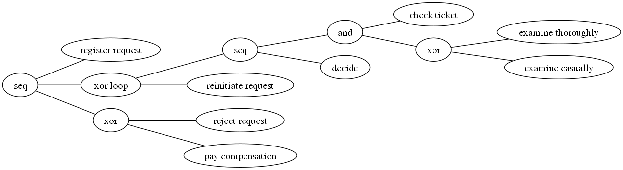
It is also possible to convert a process tree into a Petri net:
import pm4py
from pm4py.objects.petri_net.obj import Marking, PetriNet

if __name__ == "__main__":
	net: PetriNet
	initial_marking: Marking
	final_marking: Marking
	net, initial_marking, final_marking = pm4py.convert_to_petri_net(tree)
Heuristic Miner
Heuristic Miner works on the directly-follows graph, allowing it to handle noise and detect common constructs (such as dependencies and AND relationships between activities). The output is a Heuristic Net, which can then be converted into a Petri net. The paper can be found here: this link.
To apply Heuristic Miner and discover a Heuristic Net, first import the log, then generate the Heuristic Net. A variety of parameters can be explored by clicking the following button:
Inspect parameters
import pm4py
import os
import pandas
from pm4py.objects.heuristics_net.obj import HeuristicsNet

if __name__ == "__main__":
	log_path: str = os.path.join("tests", "compressed_input_data", "08_receipt.xes.gz")
	log: pandas.DataFrame = pm4py.read_xes(log_path)

	heu_net: HeuristicsNet = pm4py.discover_heuristics_net(log, dependency_threshold=0.99)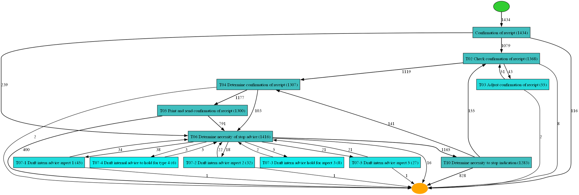
| Parameter Name | Meaning |
|---|---|
| dependency_threshold | Threshold for activity dependency (default: 0.5) |
| and_threshold | Threshold for AND relationships (default: 0.65) |
| loop_two_threshold | Threshold for loops of length 2 (default: 0.5) |
To visualize the Heuristic Net, use the code on the right:
import pm4py

if __name__ == "__main__":
    pm4py.view_heuristics_net(heu_net)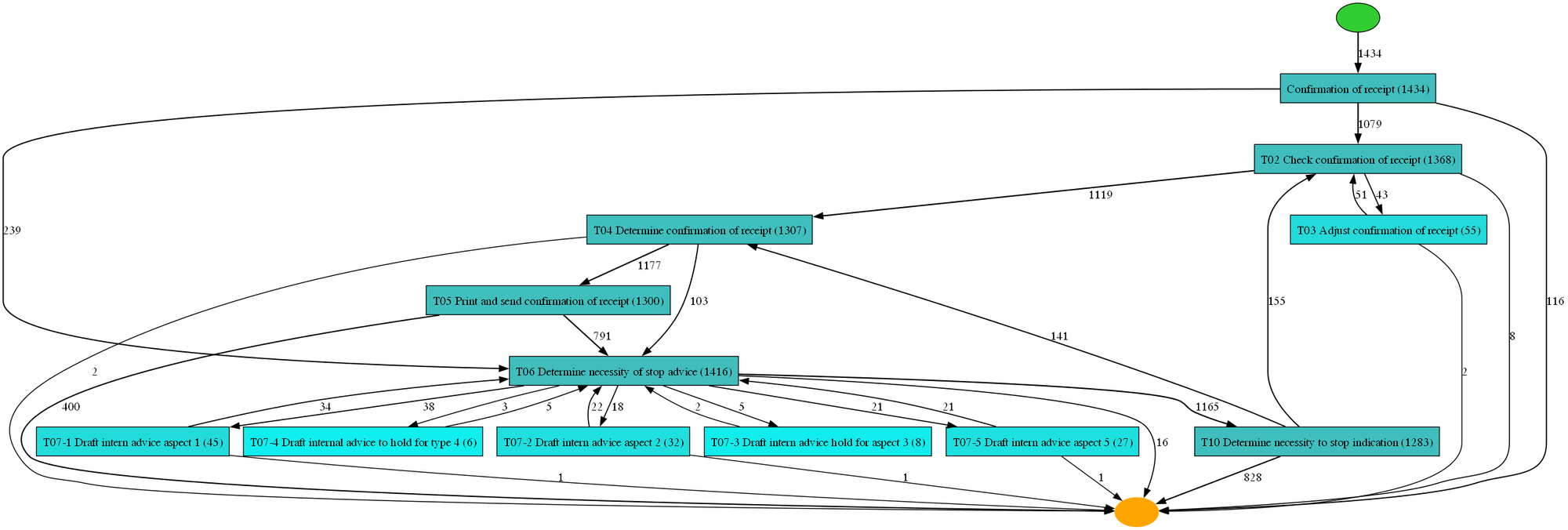
To convert the Heuristic Net into a Petri net and visualize it, use the code on the right:
import pm4py
from pm4py.objects.petri_net.obj import Marking, PetriNet

if __name__ == "__main__":
    net: PetriNet
    im: Marking
    fm: Marking
    net, im, fm = pm4py.discover_petri_net_heuristics(log, dependency_threshold=0.99)

    pm4py.view_petri_net(net, im, fm)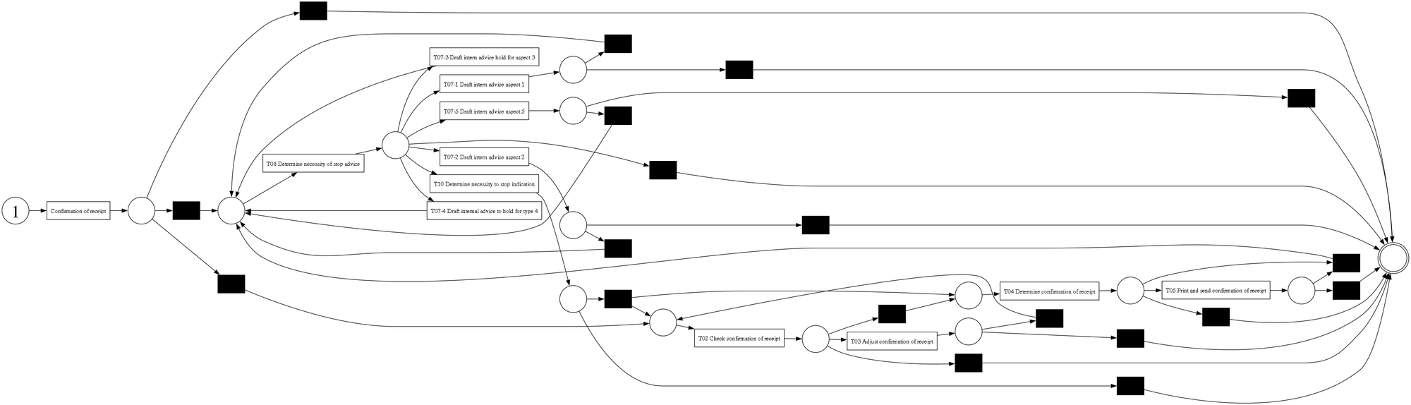
Genetic Miner
PM4Py also provides a Genetic Miner that searches for a Petri net by evolving a population of candidate models over multiple generations. Compared to directly constructive miners, it offers a more optimization-driven approach and exposes parameters such as population size, elitism, crossover, mutation, and number of generations.
In the following example, we read the running example log, discover a Petri net with the genetic miner, and then evaluate the result using token-based replay fitness and precision.
import os
import pm4py
import pandas
from pm4py.objects.petri_net.obj import Marking, PetriNet

if __name__ == "__main__":
    log: pandas.DataFrame = pm4py.read_xes(os.path.join("tests", "input_data", "running-example.xes"))
    net: PetriNet
    im: Marking
    fm: Marking
    net, im, fm = pm4py.discover_petri_net_genetic(log, population_size=10, generations=10)

    print(pm4py.fitness_token_based_replay(log, net, im, fm))
    print(pm4py.precision_token_based_replay(log, net, im, fm))
    pm4py.view_petri_net(net, im, fm)
Split Miner
Split Miner discovers a BPMN model from an event log by filtering the directly-follows graph and identifying gateway structures that balance fitness, precision, and simplicity. The reference paper is Split miner: automated discovery of accurate and simple business process models from event logs by Augusto, Conforti, Dumas, La Rosa, and Polyvyanyy.
PM4Py exposes Split Miner through pm4py.discover_bpmn_split_miner. The classic variant implements the original Split Miner, while sm2 enables the lifecycle-aware Split Miner 2.0 variant when start and end timestamp information is available.
import os
import pm4py
import pandas
from pm4py.objects.bpmn.obj import BPMN

if __name__ == "__main__":
    log_path: str = os.path.join("tests", "input_data", "running-example.xes")
    log: pandas.DataFrame = pm4py.read_xes(log_path)

    bpmn_graph: BPMN = pm4py.discover_bpmn_split_miner(
        log,
        epsilon=0.1,
        eta=0.4,
        variant="classic",
    )

    pm4py.view_bpmn(bpmn_graph)
See also the Split Miner implementation and the PM4Py examples on GitHub.
Directly Follows Graph
Process models using Petri nets have well-defined semantics: a process starts at the initial marking and ends at the final marking. Directly-Follows Graphs are another type of process model where nodes represent events/activities, and directed edges indicate that one event/activity is followed by another. You can easily add metrics like frequency or performance to these edges.
First, import the log. Then, extract and visualize the Directly-Follows Graph, decorated with activity frequencies.
import os
import pm4py
import pandas

if __name__ == "__main__":
	log: pandas.DataFrame = pm4py.read_xes(os.path.join("tests","input_data","running-example.xes"))
	dfg: dict
	start_activities: dict
	end_activities: dict
	dfg, start_activities, end_activities = pm4py.discover_dfg(log)
	pm4py.view_dfg(dfg, start_activities, end_activities)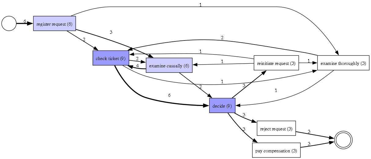
To decorate the graph with performance metrics, replace two parameters in the code:
import os
import pm4py
import pandas

if __name__ == "__main__":
	log: pandas.DataFrame = pm4py.read_xes(os.path.join("tests","input_data","running-example.xes"))
	performance_dfg: dict
	start_activities: dict
	end_activities: dict
	performance_dfg, start_activities, end_activities = pm4py.discover_performance_dfg(log)
	pm4py.view_performance_dfg(performance_dfg, start_activities, end_activities)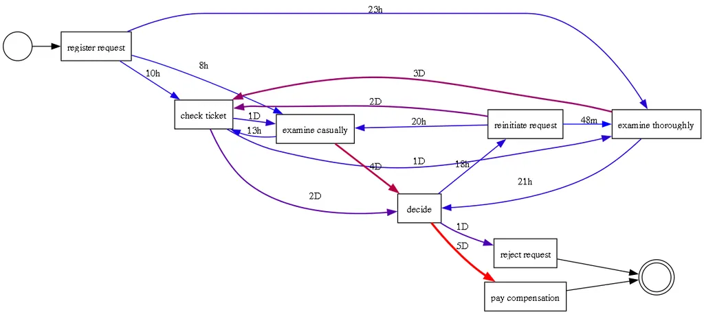
To save the DFG, for example in SVG format, use the following code:
import os
import pm4py
import pandas

if __name__ == "__main__":
	log: pandas.DataFrame = pm4py.read_xes(os.path.join("tests","input_data","running-example.xes"))
	performance_dfg: dict
	start_activities: dict
	end_activities: dict
	performance_dfg, start_activities, end_activities = pm4py.discover_performance_dfg(log)
	pm4py.save_vis_performance_dfg(performance_dfg, start_activities, end_activities, 'perf_dfg.svg')
Adding Information about Frequency and Performance
Similar to Directly-Follows Graphs, Petri nets can also be decorated with frequency or performance information. This is achieved by replaying the model and assigning frequency or performance to the paths. The variant parameter in the visualizer specifies the type of annotation to apply. The available options for the variant parameter are:
- pn_visualizer.Variants.WO_DECORATION: Default, no decoration.
- pn_visualizer.Variants.FREQUENCY: Decorates the model with frequency information from the replay.
- pn_visualizer.Variants.PERFORMANCE: Decorates the model with performance information (mean time) from the replay.
To visualize the Petri net decorated with frequency, use the following code:
from pm4py.visualization.petri_net import visualizer as pn_visualizer
from graphviz import Graph

if __name__ == "__main__":
	parameters: dict = {pn_visualizer.Variants.FREQUENCY.value.Parameters.FORMAT: "png"}
	gviz: Graph = pn_visualizer.apply(net, initial_marking, final_marking, parameters=parameters, variant=pn_visualizer.Variants.FREQUENCY, log=log)
	pn_visualizer.save(gviz, "inductive_frequency.png")
Correlation Miner
In Process Mining, event logs typically contain at least the following:
- A case identifier,
- An activity,
- A timestamp.
The case identifier links an event occurring in a system to a specific execution of a process. This association enables the use of algorithms for process discovery, conformance checking, and other process mining tasks. However, in some systems—such as those collecting data from IoT systems—it may be difficult to assign a case identifier. In these cases, performing traditional process mining is not feasible.
Correlation mining addresses this challenge by enabling the extraction of process models from event logs that lack case identifiers. These logs typically contain only:
- An activity column,
- A timestamp column.
For this explanation, we assume that a total order exists for the events (i.e., no two events share the same timestamp). Situations without a total order are more complex.
The Correlation Miner is a technique introduced by:
Pourmirza, Shaya, Remco Dijkman, and Paul Grefen. "Correlation Miner: Mining business process models and event correlations without case identifiers." International Journal of Cooperative Information Systems 26.02 (2017): 1742002.
The approach resolves the problem by solving an (integer) linear problem based on two key matrices:
- The P/S matrix: This matrix captures the order relationships between activities as recorded in the log.
- The Duration matrix: This matrix represents the duration between two activities, obtained through an optimization process.
The solution to this problem provides a set of activity pairs that are, according to the approach, in a directly-follows relationship, along with the strength of these relationships. This is referred to as the “frequency” Directly-Follows Graph (DFG).
A “performance” DFG can be derived from the Duration matrix by retaining only the entries that appear in the solution (i.e., the pairs of activities that are part of the frequency DFG).
This can then be visualized using tools such as the PM4Py DFG visualization.
For a more realistic example, we can take an existing log, remove the case ID column, and attempt to reconstruct the DFG without the case ID.
Let’s walk through an example. First, we load a CSV file into a Pandas dataframe, retaining only the concept:name and time:timestamp columns:
import pandas as pd
import pm4py
import pandas

if __name__ == "__main__":
	df: pandas.DataFrame = pd.read_csv(os.path.join("tests", "input_data", "receipt.csv"))
	df = pm4py.format_dataframe(df)
	df = df[["concept:name", "time:timestamp"]]
Next, we apply the Correlation Miner approach:
from pm4py.algo.discovery.correlation_mining import algorithm as correlation_miner

if __name__ == "__main__":
	frequency_dfg: dict
	performance_dfg: dict
	frequency_dfg, performance_dfg = correlation_miner.apply(df, parameters={"pm4py:param:activity_key": "concept:name",
									"pm4py:param:timestamp_key": "time:timestamp"})
To better visualize the DFG, we can calculate the frequency of activities:
if __name__ == "__main__":
	activities_freq: dict[str, int] = dict(df["concept:name"].value_counts())
Finally, we can visualize the DFG:
from pm4py.visualization.dfg import visualizer as dfg_visualizer
from graphviz import Graph

if __name__ == "__main__":
	gviz_freq: Graph = dfg_visualizer.apply(frequency_dfg, variant=dfg_visualizer.Variants.FREQUENCY, activities_count=activities_freq, parameters={"format": "svg"})
	gviz_perf: Graph = dfg_visualizer.apply(performance_dfg, variant=dfg_visualizer.Variants.PERFORMANCE, activities_count=activities_freq, parameters={"format": "svg"})
	dfg_visualizer.view(gviz_freq)
	dfg_visualizer.view(gviz_perf)
Upon visualizing the DFG, we can confirm that the Correlation Miner successfully identified a clear main path in the process.
The Correlation Miner offers several variants, each with its own characteristics:
| Variant | Description |
|---|---|
| Variants.CLASSIC | Calculates the P/S matrix and the Duration matrix using the entire event list in a traditional manner. |
| Variants.TRACE_BASED | Calculates the P/S matrix and Duration matrix on a trace-by-trace basis using a classic event log and merges the results. This variant produces a more understandable model compared to the classic DFG. |
| Variants.CLASSIC_SPLIT | Calculates the P/S matrix and Duration matrix on the entire event list but splits it into chunks to speed up the computation. While this results in a less accurate model than the CLASSIC variant, the computation is faster. The default chunk size is 100,000 events. |
Temporal Profile
PM4Py includes an implementation of the temporal profile model, which is described in:
Stertz, Florian, Jürgen Mangler, and Stefanie Rinderle-Ma. "Temporal Conformance Checking at Runtime Based on Time-infused Process Models." arXiv preprint arXiv:2008.07262 (2020).
The temporal profile measures, for each pair of activities in the log, the average time and standard deviation between events containing those activities. The time is measured between the completion of the first event and the start of the second event. This model assumes an interval log, where events have two timestamps.
The output of the temporal profile discovery is a dictionary where each activity pair (represented as a tuple) is associated with two values: the average time and the standard deviation of the time interval between the events.
An example of temporal profile discovery is provided below. First, we load an event log and apply the discovery algorithm.
import pm4py
from pm4py.algo.discovery.temporal_profile import algorithm as temporal_profile_discovery
import pandas

if __name__ == "__main__":
    log: pandas.DataFrame = pm4py.read_xes("tests/input_data/running-example.xes")
    temporal_profile: dict = temporal_profile_discovery.apply(log)
Several parameters can be used to customize the execution of the temporal profile discovery:
| Parameter Key | Type | Default | Description |
|---|---|---|---|
| Parameters.ACTIVITY_KEY | string | concept:name | The attribute to use as the activity. |
| Parameters.START_TIMESTAMP_KEY | string | start_timestamp | The attribute to use as the start timestamp. |
| Parameters.TIMESTAMP_KEY | string | time:timestamp | The attribute to use as the timestamp. |
Local Process Models
Local Process Models aim to find frequent and recurring patterns describing parts of the event log, usually focusing on a subset of activities.
They were first introduced in "Mining local process models" (2016) by Tax, N., Sidorova, N., Haakma, R., & van der Aalst, W. M. Journal of Innovation in Digital Ecosystems, 3(2), 183-196.
In contrast to episode and sequential pattern mining, Local Process Models are represented by Process Trees and can therefore model loops and exclusive choices alongside sequences and concurrency.
The algorithm returns a list of process trees together with their quality metrics. Confidence, language fit, determinism, and coverage range from 0 to 1. Instead of the normalized support metric introduced in the paper, PM4Py exposes frequency directly as a count of model executions.
- Frequency: Measures how often a Local Process Model is executed in the event log. Note that per trace the model can be executed multiple times.
- Confidence: Measures, per activity in the model, the ratio of events which are part of model executions. The harmonic mean over all activities in the model is returned.
- Language fit: Describes the precision of the model by calculating how many of the allowed traces in the Local Process Model are actually executed.
- Determinism: Measures the amount of choices in the state space of the model. Fewer choices lead to higher determinism values.
- Coverage: The ratio of events in the log that stem from activities used in the model.
Evaluating a large number of these process models is costly. Limiting the activities considered through the selected_activities argument leads to a smaller search space and can improve performance. If this argument is omitted, all activities in the log are considered.
Several parameters can be used to customize the execution of the local process model discovery:
| Parameter Key | Type | Default | Description |
|---|---|---|---|
| Parameters.CASE_ID_KEY | string | case:concept:name | Key used to correlate events into cases. |
| Parameters.ACTIVITY_KEY | string | concept:name | Key to use within events to identify the underlying activity. |
| Parameters.TIMESTAMP_KEY | string | time:timestamp | Key to use within events to identify the timestamp. |
| Parameters.FREQUENCY_THRESHOLD | int | 20 | Positive integer frequency threshold. |
| Parameters.CONFIDENCE_THRESHOLD | float | 0.7 | Confidence threshold between 0 and 1. |
| Parameters.DETERMINISM_THRESHOLD | float | 0.5 | Determinism threshold between 0 and 1. |
| Parameters.LANGUAGE_FIT_THRESHOLD | float | 0.3 | Language fit threshold between 0 and 1. |
| Parameters.COVERAGE_THRESHOLD | float | 0 | Coverage threshold between 0 and 1. |
| Parameters.MAX_ITERATIONS | int | 3 | Maximum number of iterations of the search algorithm. In each iteration 'i' Process Trees with exactly 'i' activities are considered. |
| Parameters.MAX_NUMBER_OF_MODELS | int | None | The maximum number of models to be returned. Can be used to restrict the solve time. |
| Parameters.MULTI_PROCESSING | boolean | False | Whether to use multiprocessing. |
| Parameters.TIME_LIMIT | float | None | Soft time limit for the computation, in seconds. The current model (or multiprocessing batch) is completed before the search stops. |
| Parameters.PROGRESS_BAR_TYPE | string | explored_lpms | Default value explored_lpms shows the number of explored LPMs in each iteration. Use found_lpms to show a progress bar for the number of LPMs found so far in relation to MAX_NUMBER_OF_MODELS. Otherwise, use None to hide the progress bar. |
Here is a small example of local process model mining.
import os
import pm4py
import pandas
from pm4py.algo.discovery.local_process_models.algorithm import find_local_process_models
from pm4py.algo.discovery.local_process_models.variants.classic import Parameters

if __name__ == "__main__":
    log_path: str = os.path.join("logs", "road_traffic_fine_management.xes")
    log: pandas.DataFrame = pm4py.read_xes(log_path)

    lpms = find_local_process_models(
        log,
        selected_activities=[
            "Insert Date Appeal to Prefecture",
            "Send Appeal to Prefecture",
            "Receive Result Appeal from Prefecture",
            "Notify Result Appeal to Offender",
            "Appeal to Judge",
        ],
        parameters={
            Parameters.FREQUENCY_THRESHOLD: 25,
            Parameters.TIME_LIMIT: 60,
            Parameters.MAX_ITERATIONS: 3,
            Parameters.PROGRESS_BAR_TYPE: "explored_lpms",
            Parameters.MAX_NUMBER_OF_MODELS: 100,
        },
    )

    if lpms:
        # Results are returned in discovery order; select one to inspect.
        process_tree, metrics = lpms[-1]
        pm4py.view_process_tree(process_tree)
Each result is a tuple containing a standard process tree and a LocalProcessModelStats object. Here is an example of a local process model that could be found:

